Big O Notation Basics for Web Developers

Big O notation

“Big O notation is a mathematical notation that describes the limiting behaviour of a function when the argument tends towards a particular value or infinity. It is a member of a family of notations invented by Paul Bachmann, Edmund Landau, and others, collectively called Bachmann–Landau notation or asymptotic notation.”

— Wikipedia’s definition of Big O notation

In other words one can say that Big O notation is a mathematical notation for describing the performance or complexity of an algorithm.

Why this is important for web developers is because it enables a web developer to determine how efficient different approaches to solving a problem are, as Big O Notation is a way to represent how long an algorithm will take to execute.

Further it will allow the early detection of potential performance and optimisation issues.

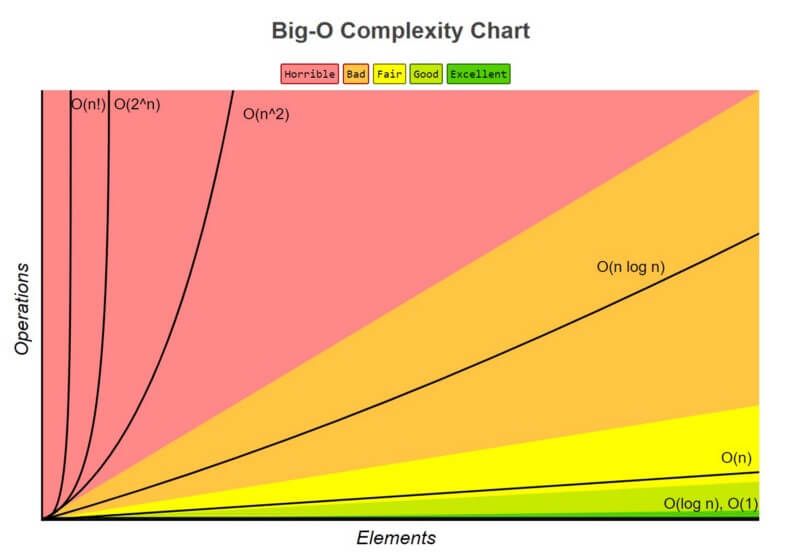
Complexity Growth Illustration

Here are some common types of time complexities in Big O Notation.

O(1) - Constant time complexity
O(n) - Linear time complexity
O(log n) - Logarithmic time complexity
O(n^2) - Quadratic time complexity

O(1)

Constant time algorithms will always take same amount of time to be executed. The execution time of these algorithm is independent of the size of the input.

A good example of O(1) time is accessing a value with an array index.

O(n)

An algorithm has a linear time complexity if the time to execute the algorithm is directly proportional to the input size n. Therefore the time it will take to run the algorithm will increase proportionately as the size of input n increases.

A good example is finding a CD in a stack of CDs or reading a book, where n is the number of pages. Another good example is that of using linear search.

O(log n)

An algorithm has logarithmic time complexity if the time it takes to run the algorithm is proportional to the logarithm of the input size n.

An example is binary search, which is often used to search data sets.

O(n^2) (The Quadratic Function)

An algorithm has quadratic time complexity if the time to execution it, is proportional to the square of the input size. Therefore if the input size is 2, then the required steps are 4. If the input is size 8, it will take 64, and so on. A good example of this is checking to see whether there are any duplicates in a deck of cards.

You will encounter quadratic time complexity in algorithms involving nested iterations, such as nested for loops. In fact, the deeper nested loops will result in O(n^3), O(n^4), etc.

Other examples of quadratic time complexity include bubble sort, selection sort, and insertion sort.

Below is an example of an O(n²) algorithm bubble sort algorithm:

Bubble sort compares adjacent elements. It starts with the first two elements and it interchanges them if the first element is larger than the second element. It repeats the same steps until it reaches the end of the array. Again the same steps will repeat from the i+1 element. The greater input, the greater the steps needed to complete the sort.

Linear Search versus Binary Search Algorithm

A linear search scans one item at a time, without jumping to any item.

The worst case complexity is O(n), sometimes known an O(n) search
Time taken to search elements keep increasing as the number of elements are increased.

A binary search however, cut down your search to half as soon as you find middle of a sorted list.

The middle element is looked to check if it is greater than or less than the value to be searched.
Accordingly, search is done to either half of the given list

When the amount of data is small, this search is fast. It's easy but work needed is in proportion to the amount of data to be searched. Doubling the number of elements will double the time to search if the desired element is not present, which can greatly increase the inefficiency of the search if the data set is large.

However, binary search is efficient for a larger data set. But the table must be sorted for binary search.

Therefore overall, one could suggest that binary search is faster than linear search except for small arrays. However, the array must be sorted first to be able to apply binary search.

The time complexity of linear search is O(n) whereas binary search has time complexity O(log n).

Fibonacci sequence

A Fibonacci sequence is a group of numbers where you determine the next number in the sequence by adding the previous two numbers in the sequence together.

E.g. (Fibonacci numbers: 1, 1, 2, 3, 5, 8, 13, 21, 34 ... )

Below is an example of a recursive function which displays the first 5 numbers of the sequence:

Here, instead, is an example of an iterative function which displays the first 5 numbers of the sequence:

One could suggest here that the for the iterative approach, the amount of space required is the same for fib(6) and fib(100), i.e. as N changes the space/memory used remains the same. Hence it’s space complexity is O(1) or constant.

For Fibonacci recursive implementation or any recursive algorithm, the space required is proportional to the maximum depth of the recursion tree, because, that is the maximum number of elements that can be present in the implicit function call stack.

As you can see the maximum depth is proportional to the N, hence the space complexity of Fibonacci recursive is O(N).So when doing the recursive implementation of Fibonacci algorithm, you are adding redundant calls by recomputing the same values over and over again.

Therefore, one could suggest that the iterative 0(1) approach would be the more efficient solution to the problem at hand.